Wild Fig Multi Strategy Hedge Fund Q2 Investor Update


Introduction
“The most important quality for an investor is temperament, not intellect” – Warren Buffett. During a quarter filled with a barrage of headlines, investors who remained calm, disciplined and rational in the face of market fluctuations and uncertainties were, for the most part, better off. Quarter 2 headlines were driven by Trump 2.0 and his policies surrounding the US tariff trade stance, the ensuing widespread global market sell-off and the subsequent 90-day pause that triggered a sharp reversal of these losses. Despite the rollercoaster of events, indices moved higher over the quarter. In dollar terms: S&P500 (10.8%); Nasdaq 100 (17.9%); MSCI ACWI (11.5%); Hang Seng (5.7%) and EuroStoxx (1.4%).
US equity markets wrapped up the quarter at all-time highs despite the drawdown in April on the back of Trump’s Liberation Day tariff announcement. Gains in the US were led by the information technology and communication services sectors as investor appetite for some of the “Magnificent 7” stocks reignited, while stocks with exposure to artificial intelligence staged a strong recovery after some weakness earlier in the year. US shares were also supported by generally robust corporate earnings for Q1. Dollar weakness continued during the quarter, with the greenback posting its weakest first six months of the year since 1973 – this as President Donald Trump’s economic policies have prompted global investors to question the currency’s “safe haven” status. The Federal Reserve kept interest rates on hold at 4.25-4.50%.
The strained US-China relationship weighed on Chinese growth expectations and commodity demand. The ripple effects were felt globally, with industrial metals under pressure. The overarching macro theme for China in 2025 will be rising external hostilities amid prolonged domestic economic hardship. Key focus in the third quarter will be the effective tariffs imposed by the US and the reciprocation of Chinese officials.
Domestically, the JSE All Share Index (ALSI) increased by 10.2% (in ZAR). Signals from the SARB and Treasury that they aim to shift the inflation target closer to 3% sparked a meaningful bond rally, taking the benchmark 10-year yield below the technical 10% level and supporting the rand, appreciating by 3.3% and ending the quarter at R17.71 against the US dollar. Political tension within the GNU eased after another fallout between the ANC and DA, resolving its cabinet spat when President Ramaphosa asked coalition partner DA to nominate a new deputy minister, quelling fears of a breakdown. Separately, South Africa ticked off the final Financial Action Task Force milestones, an on-site review later this quarter should pave the way for removal from the grey list in October.
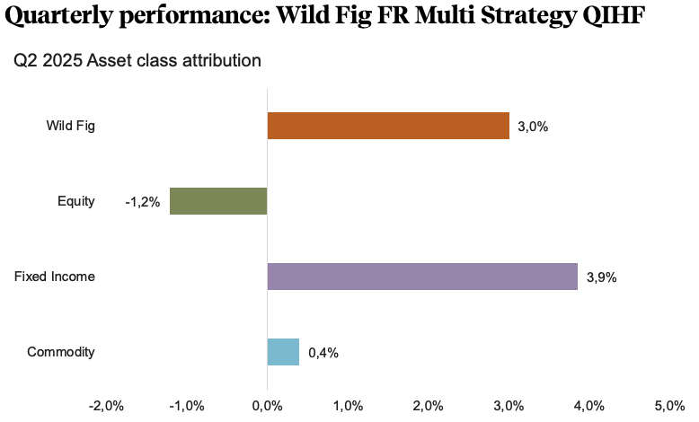
In summary, the Fairtree Wild Fig Multi Strategy FR QIHF, “Wild Fig”, our flagship multi-strategy balanced hedge fund, delivered a positive return for the quarter (+3.0%), which helped offset the drawdown in Q1. The fund is roughly flat year to date. The fund remains true to its investment objective of compounding clients’ capital over the long term. We thank you for entrusting us as stewards of your capital.
Wild Fig Multi Strategy
Portfolio Management Team
Source: Fairtree Bloomberg.
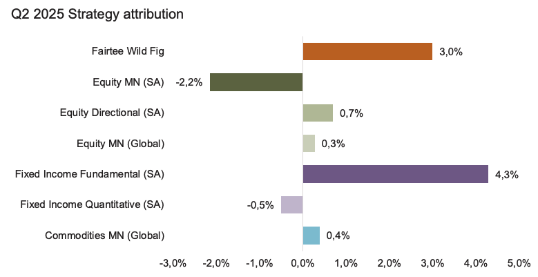
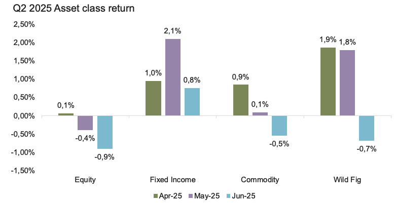
The positive performance during the second quarter of 2025 was attributable to positioning in Fixed Income (more specifically our SA Fundamental strategy) and Commodities, whilst positioning in Equities detracted.
Source: Fairtree, Bloomberg.
In aggregate, equities generated a negative return for the quarter on the back of positioning in our South African equity market-neutral construct. The Fund’s positioning in consumer discretionary, healthcare and the materials sectors detracted from the Fund’s performance. However, the Fund’s positioning in the financials and communication services partially offset the detraction, in addition to small gains in our directional and global equity sleeves.
Although the SARB has been reluctant to cut rates on the back of global policy uncertainty (trade war) and the impact that potential tariffs could have on inflation, the Fixed Income Fundamental (SA) strategy has held the view for a prolonged period that there aren’t enough rate cuts currently being priced into the market. In addition to this, the team has also held the view that the SA bond yields should rally based on the SARB’s commitment to a lower inflation target and National Treasury’s commitment to fiscal consolidation in the third budget. As a result, the positioning in the FRAs and the belly of the bond curve contributed significantly to the asset class performance this quarter.
Within the Commodities strategy, positive contributions came from pair trades within our Origin Differential and Demand Substitution risk buckets, while unsustainable margins detracted from performance over the quarter. Pairs within the Producer Return on Investment risk Bucket ended the quarter flat.
Source: Fairtree, Bloomberg.
Quarterly insights: In search of capital efficiency
Interest in hedge funds has soared over the past 20 years. Changes in CISCA regulations and the advent of Retail Investor Hedge Funds (RIHFs) have provided further tailwinds to investor demand locally as investors seek to diversify their portfolios with a particular focus on downside protection in tumultuous markets.
A question allocators consistently grapple with is how much they should allocate to hedge funds (or other deemed riskier alternative asset classes), seeing as it is assumed common knowledge (albeit somewhat naively, yet unintentionally) that hedge funds are riskier than other, more traditional investments, commonly referred to as “long-only” investments.
Volatility drags
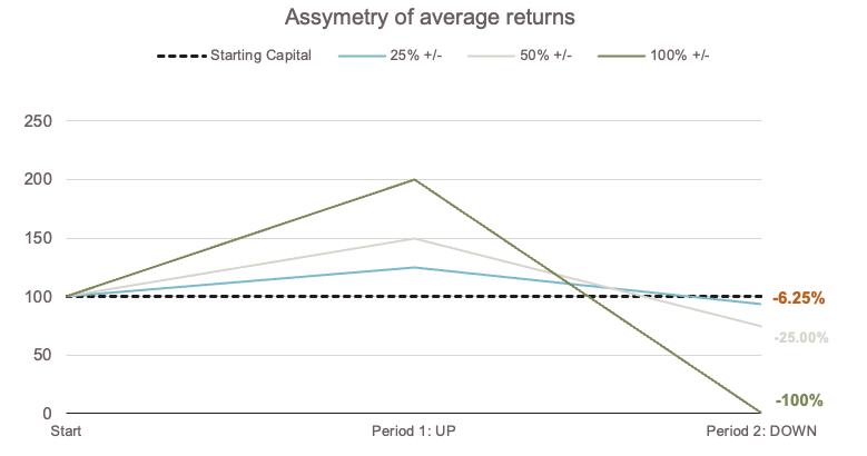
Volatility of returns, measured by the standard deviation of a return series, is seen as an industry-wide standard for comparing investment risk profiles. While “risk” is a nuanced concept, most rational investors accept the widely held view that volatility is detrimental to compounding returns. This is because, over time, the asymmetry of returns introduces what is known as volatility drag, where large fluctuations reduce the compounded growth rate of capital, even if the average (arithmetic) return is constant. An investor earning +25% followed by -25%, is down -6.25%; +50% up and then -50% down, leaves the investor -25% down overall, and (key to understanding risk-investments) a +100% return followed by a 100% loss, wipes out the fund completely. Importantly, all these investors earned the same 0% average return over time.
Source: Fairtree, Illustrative
Volatility & capital efficiency
However, this view primarily applies at the portfolio level. When it comes to holding or strategy level, high-volatility strategies can offer compelling capital efficiency, even if their standalone compound returns are lower.
Capital efficiency refers to the ability of an investment strategy to generate the highest possible return (risk-adjusted), or portfolio utility, per unit of capital allocated. In other words, it’s based on the premise of how effectively limited capital is used to contribute to overall portfolio performance, particularly in terms of overall return, diversification, and risk contribution.
In the context of portfolio construction, capital efficiency is not just about maximising returns, but about maximising the value extracted from each rand (or unit) allocated, relative to its risk, correlation, and opportunity cost.
As a summary, a strategy is said to be capital efficient if it delivers:
- High risk-adjusted returns (e.g. high Sharpe or information ratio),
- Strong diversification benefits (e.g. low correlation with core holdings),
- Or allows a smaller allocation to achieve the same impact, thereby freeing up capital for other uses.
This becomes particularly important in alternative, or specifically hedge fund investing, where leverage, risk budgeting, and position sizing play critical roles. Allocating to a high-volatility, uncorrelated strategy that delivers similar marginal utility to a lower-volatility strategy, whilst importantly using less capital, is more capital efficient, even if the standalone compound return is lower.
Nuts and bolts – a practical example
What defines an “alternative” investment is quite broad and is loosely defined as anything outside the traditional long-only or listed investment universe, such as listed equity and bonds. However, a key differentiating factor and relevant to this report is that when considering alternatives, an investor has an unconstrained toolkit available, which includes the prudent application of leverage. The application of leverage is a crucial part of a capital-efficient strategy, as the trade-off between volatility and efficiency is directly related.
By way of example, using a widely used hedge fund strategy, “Equity Long/Short”, a manager attempts to identify opportunities and profit from both increases and decreases in absolute positions, thereby isolating stock-specific performance from that of the market.
Practically, this could be executed as a portfolio using one hundred rand (R100) to begin with and deploying this in various specific opportunities – either by taking long (buying the asset) or short positions (borrowing and selling the asset with the intent of profiting from the decrease in value). The portfolio return can simplistically be defined as:
= Return on Longs + Return on Shorts
Seeing as a hedge fund executes trades using leverage or thus posting margin by buying a derivative of the individual equity securities (not the actual cash equities), cash is deposited in a margin account with a prime broker who executes the trade on behalf of the fund. The portfolio return can roughly be defined as:
= Cash return + Risk component return, or
= Cash return + (Return on Long + Return on Short)
The volatility (or “σ “) of the portfolio return, over a risk-free (cash component), will thus be the volatility of the risk component return, as cash sits idle generating the risk-free rate. However, when applying leverage (L x times levered), as one commonly does in most hedge fund trade executions, your R100 now turns into L x R100, or LR100 both long and short, and the returns are calculated as:
= Cash return + L *(R100Long + R100Short), or
=Cash return + (LR100Long + LR100Short)
When calculating the portfolio volatility, however, the new volatility is merely the volatility multiplied by the leverage factor (L * σ). For simplicity, we ignore transaction and trading costs. The interesting result is that even though the CAGR over time compounds, the portfolio’s Sharpe remains the same. Consequently, to achieve the same risk-adjusted return on a portfolio level, but at lower risk, an investor can simply cap the allocation towards the risk component.
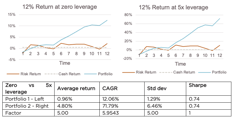
Source: Fairtree. Illustrative. Both Portfolio 1 and Portfolio 2 target a 12% nominal return over the 12-periods. Average return is the average of all the period-specific returns, including leverage where applicable.
Increase in portfolio outcome
Another way to frame this is through the lens of a consistent Sharpe ratio – i.e., the additional return an investor is compensated for by the incremental increase in risk. When considering the capital efficiency ratio as optimal use of incremental capital, it can be expressed as:
Capital efficiency = Marginal portfolio utility / Capital allocated.
If we assume:
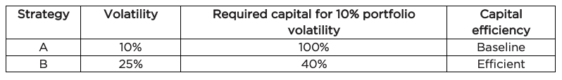
- Target volatility = σtarget = 10%
- Strategy volatility = σstrategy
- Capital allocation weight = ω
And, assuming:
- Both strategies are uncorrelated with other positions in the portfolio,
- The portfolio consists entirely of this single strategy at a scaled weight,
Then we can conclude the following relationship:
σportfolio= ω x σstrategy
And solving for the required strategy capital weight:
ω = σtarget / σstrategy
As our portfolio volatility target is 10%, Strategy A equates to an allocation of 100% (ω =10% / 10% =1.0 or 100% capital allocation). Whereas, to achieve the same target volatility of 10%, Strategy B has a weighting of 40% (ω =10% / 25% =0.4 or 40% capital allocation). Strategy B, despite being more volatile, requires less capital to reach the same target contribution to portfolio volatility, to achieve the same Sharpe (or risk-adjusted) outcome. The freed-up leftover 60% of capital can be redeployed to other, uncorrelated or complementary return sources, thereby improving the overall portfolio return. This is the essence of capital efficiency: not how much you earn in isolation, but how much portfolio utility you get per unit of capital put to work.
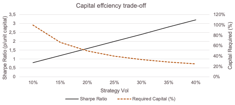
Source: Fairtree. Illustrative. Portfolio Vol fixed at 10% to calculate the Sharpe p/unit capital. Sharpe Ratio of strategies fixed at 0.8 to calculate the capital required %.
A binary example
A simple outcome from a binary lens is edifying. Imagine you face a binary set of possible outcomes on an investment: a 2/3 (or 66.66%) chance you double your money (+100%) and a 1/3 chance (or 33.33%) you lose it all (-100%). And assume this investment is uncorrelated with the rest of the investor’s portfolio, three things should be obvious:
- The return an investor can expect to generate is equal to the probability weighted average of the outcomes, i.e., Expected return (ERp) = (P1×ER1) + (P2×ER2), or, in other words = 33.33%
- Even though there is a strong positive expected return (33.33%), with a strong convex payoff, the multi-period compound return on this investment viewed alone will eventually be -100%, in other words, wipes out the investor, as explained in the introduction. Thus, putting your whole portfolio in this wouldn’t be such a good idea, and viewed in isolation, there is a high degree of capital risk.
- Conversely, any rational investor should put part of their portfolio in this investment, as a very positive expected return and -100% on a small part of a diversified overall portfolio is eminently survivable and improves the total portfolio outcome.
When you lose (or win), you just reload the allocation and rebalance, and, over time, the trade-off will be favourable with an attractive compounded growth component to the portfolio. The key consideration, however, is the ability to reload, or from an investment perspective, rebalance.
Rebalancing and compound growth over time
The capital efficiency trade hinges on the ability to rebalance a portfolio, or benefit from the benefit of the volatility of the return series over time. This trade-off off however, is not linear, as in theory (i.e. no transaction costs, drawdown, versions, etc.) at a constant Sharpe ratio, the efficiency scale linearly. However, in practice, actual portfolio utility is non-linear.
By way of example, let’s look at a portfolio of multiple asset classes and theoretical but reasonable assumptions around expected returns, volatility, etc.
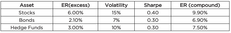
Source: Fairtree. Note, assume cash is 5% with E[excess] below being the expected return of each asset over cash. Expected returns = ER(excess) – ½ vol squared. Correlation between stocks and bonds is assumed as 0.30, and the correlation between both stocks and bonds, with hedge funds, is assumed to be zero.
We can calculate the expected compound return as:
Compound return ≈ Arithmetic return (ERexcess + ERcash) – ½ σ2
We assume the correlation of stocks to bonds to be 0.30 and the correlation of the hedge fund with both stocks and bonds to be 0.00 (an ideal world situation, for illustrative purposes). This second term is a mathematical version of the intuitive “volatility drag” discussed earlier with basic examples, and is quadratic in nature. Thus, over time, high-volatility strategies lose more to compounding drag and reduce the compound growth.
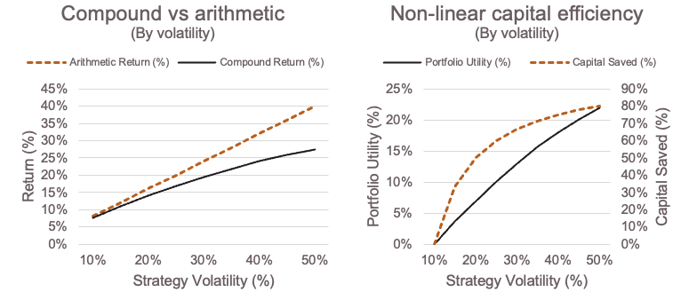
Source: Fairtree. Illustrative.
With repeat rebalancing between low-correlated, high-vol strategies, an investor extracts volatility as return:
Utility = f (Volatility, Correlation, Rebalance Frequency)
This function is non-linear, as with heightened levels of dispersion, rebalancing and tail-event control improve utility over time.
Using constrained mean-variance optimisation, we can determine the optimal blend of asset classes by solving for an optimal portfolio, defined here as the highest expected compound return with a maximum allowable volatility of 10% and not allowing any leverage (so portfolio weights must add to less than or equal to 100%), and initially ignoring the addition of a hedge fund, or risk-component, allocation:
Given, using mean-variance optimisation:
Portfolio return = ω⊤ μ
Where:
- ω is the vector of portfolio weights
- μ is the vector of expected returns for each asset
And subject to the following:
- Portfolio variance constraint (target volatility = 10%): ω⊤ Σω =σ2target =0.01
Where:
- Σ is the covariance matrix of asset returns
- σtarget is the target portfolio volatility of 10%
- Capital constraint (fully invested): ∑ni=1 ωi = 1
- Long-only constraint: ωi ≥0 for all i
We solve for the optimal portfolio as:
- Stocks/bonds/hedge funds = 58/42/0
- E[compound] = 8.9%
- Total volatility = 10%
Now, calculating the same optimised portfolio weights, but allowing the 10% vol hedge fund allocation into the asset mix:
- Stocks/bonds/hedge funds = 62/0/38
- E[compound] = 9.3%
- Total volatility = 10%
Not surprisingly, the optimisation gets better when you allow an additional asset (40 bps per annum improvement). What may be a bit surprising is that the hedge fund almost completely replaced the bond allocation. With these assumptions, the hedge fund is essentially just a better version of bonds: a similar Sharpe ratio as bonds but at zero correlation to the very volatile equity portion. And, because you can’t lever (total weights = < 100%), there’s no room for bonds anymore.
The duality between volatility and leverage
First, let’s assume the same asset mix but that the hedge fund return generates a 25% volatility (i.e., expected excess return of 7.5%), the optimisation returns the following:
- Stocks/bonds/hedge funds = 48/28/24
- E[compound] = 9.8%
- Total volatility = 10%
The results are a sizeable allocation to the hedge funds (though a bit less than half as much as when the hedge funds were at 10% volatility, as the optimisation is controlling the hedge fund volatility by the amount it invests). You now make 90 bps a year more than not having any access to the hedge fund alternative, and 50 bps more a year than when the hedge funds were only available at 10% volatility. Perhaps most interesting, though, is that the bond allocation is resurrected. Bonds, within these assumptions, are a pretty good investment, just not as good as a hedge fund (same Sharpe but more correlation to equities makes them worse). When the hedge fund isn’t very volatile, you need to allocate a lot of dollars to it, and that boxes out the bonds. But when the hedge fund is more volatile, you don’t want or need as high an allocation, and there’s room again in the portfolio for bonds, which still have low correlation to equities and none to hedge funds, raising the compound return and Sharpe of the full portfolio.
Lastly, when using the benefit of increased volatility but when adding the benefit of leverage (i.e. relaxing the no leverage constraint and note that you can use any volatility number, as when you can lever or de-lever to essentially optimise for capital efficiency), the following is the result:
- Stocks/bonds/hedge funds = 43/52/22
- E[compound] = 9.8%
- Invested at = 118% (i.e., now levered at 1.18x)
- Total volatility = 10%
The same compound return as the prior case – to be expected. Similar to when you have the 25 vol hedge fund allocation, you are not very constrained at all by the “no leverage” rule. In fact, if the volatility of the hedge fund were higher than 25, the no-leverage and leverage-allowed cases would be precisely the same (as you don’t need any leverage when the assets are sufficiently volatile on their own). Another way to frame the same concept is to do the same optimisation, but with the 10% volatility hedge funds (still allowing leverage):
- Stocks/bonds/hedge funds = 42/53/56
- E[compound] = 9.8%
- Invested at = 151% (i.e., now levered at 1.51x)
- Total volatility = 10%
Same exact result, but you need more leverage. The optimiser is simply putting 2.5x more (10 vs. 25 vol) into the hedge funds. Allowing leverage is equivalent to choosing the level of volatility you desire.
Conclusion
High-volatility strategies that use less capital unlock exponential optionality, with three distinct benefits: i) capital can be reallocated to other high-alpha or defensive strategies, ii) in crisis periods, having reserve capital allows for opportunistic deployment (tactical buying opportunities), iii) which makes capital efficiency convex in value as portfolio complexity and opportunity set grow.
Higher volatility investment strategies, when distinctly uncorrelated and thoughtfully constructed in terms of portfolio construction and rebalancing discipline, can enhance overall portfolio efficiency more than their lower volatility counterparts. When constructing the optimal portfolio, however, an investor should target a higher capital efficiency, and therefore a smaller allocation, but counterintuitively actively seek out higher volatility if they are able to stomach the short-term volatility. Higher-vol alternatives investment options can be “better” not despite the vol, but because of it, if sized correctly in a diversified portfolio.
Topics
Disclaimer
Fairtree Asset Management (Pty) Ltd is an authorised financial services provider (FSP 25917). Collective Investment Schemes in Securities (CIS) should be considered as medium-to-long-term investments.
The value may go up as well as down and past performance is not necessarily a guide to future performance. CISs are traded at the ruling price and can engage in scrip lending and borrowing. A schedule of fees, charges and maximum commissions is available on request from the Manager. A CIS may be closed to new investors in order for it to be managed more efficiently in accordance with its mandate. Performance has been calculated using net NAV to NAV numbers with income reinvested. The performance for each period shown reflects the return for investors who have been fully invested for that period. Individual investor performance may differ as a result of initial fees, the actual investment date, the date of reinvestments and dividend withholding tax. Full performance calculations are available from the manager on request. There is no guarantee in respect of capital or returns in a portfolio. Prescient Management Company (RF) (Pty) Ltd is registered and approved under the Collective Investment Schemes Control Act (No.45 of 2002). For any additional information such as fund prices, fees, brochures, minimum disclosure documents and application forms please go to www.fairtree.com
We are Fairtree
Subscribe to our newsletter
Stay informed with the latest insights and updates. Subscribe to our newsletter for expert analysis, market trends, and investment strategies delivered straight to your inbox.

"*" indicates required fields

FAIRTREE INSIGHTS
Your may also be interested in
Explore more commentaries from our thought leaders, offering in-depth analysis, market trends and expert analysis.

Fairtree Global Flexible Income Plus Fund Q2 2025 Commentary
After the very slow start for US equities during the first quarter, and the superior performance emanating from the EU and the UK, the second quarter witnessed a turnaround in fortunes with the tech-heavy NASDAQ delivering its fourth-best quarterly performance number over the past 18 years.

Fairtree Balanced Prescient Fund Q2 2025 commentary
We anticipate continued macroeconomic uncertainty throughout 2025. Global investors remain cautious amid evolving geopolitical tensions and shifting trade policies.


Fairtree Global Equity Fund Q2 2025 Commentary
US equities ended the quarter 11.2% higher; however, they experienced pronounced volatility following President Donald Trump’s ‘Liberation Day’ announcements of tariffs on imported goods.
About you…
By proceeding, I confirm that:
- To the best of my knowledge, and after making all necessary inquiries, I am permitted under the laws of my country of residence to access this site and the information it contains; and
- I have read, understood, and agree to be bound by the Terms and Conditions of Use described below.
- Please beware of fraudulent Whatsapp groups pretending to be affiliated with Fairtree or Fairtree staff members.
If you do not meet these requirements, or are unsure whether you do, please click “Decline” and do not continue.